 Post Feed
Making of »nano«
In the last two months, there has been a fair (but not overwhelming) amount of media awareness around the Evoke Alternative Platform winner demo, »nano«. I’ve been interviewed for a minor German internet portal and for a major German Mac magazine and received almost exclusively good ratings on pouët.net. Finally, a few weeks ago, Gasman (a well-respected scener) started a thread about it in the iPodLinux forums. There were numerous people wondering about how it’s possible to do real-time 3D graphics on the iPod nano. To answer these questions once and for all, I’ve taken much time to write this very long post that really should contain all relevant information.
Idea and design
 I’ll answer the most important (and most frequent) question first: Why does someone make a demo on something like an iPod? It’s simple: Because it’s possible! The demoscene is all about exploring the limits of what’s possible on any given hardware. So, if it is possible to make a demo on an obscure platform, it’s only a question of time until someone takes a chance and does it. Regarding the iPod nano, I just happened to be the first guy to do it.
Strictly speaking, »nano« isn’t the first iPod demo. It’s only the first demo on the iPod nano, or color iPods in general. There has already been a demo on the older monochrome hard disk-based models (1G-4G): Podfather by Hooy-Program, coded by Gasman (the very guy who started the discussion on »nano« in the iPodLinux forums :). While this demo was an outstanding achievement by itself, the content was rather »old-schoolish« and seemed to me more like a proof of concept than a modern, well-designed demo.
To make a long story short, I wanted to do better :) I wanted to do a demo that is not only good because it runs on the second smallest device that has ever been »demoed« (the smallest one being the Nintendo Pokémon Mini). It also should be a demo I’d personally like as such, it should be new-school. It should have a consistent theme and mood, pleasing graphics, a good soundtrack and all that. I actually strived for TBL excellence, although I knew from the start that I’m going nowhere near that. But hey, it’s always good to have dreams :)
The problem with all these wishes and goals was that I didn’t have a clear idea of the general topic of the demo. Finally, I settled for the obvious one: It’s a demo for a iPod nano, so I made »nano« the title and theme of the project, too. At first, I only wanted to show some unsorted microscopic, nano-technologic, biologic or chemical stuff. Later on, I refined that idea into its final shape: A journey from very large-scale stuff like galaxies and planets down to real nanoscopic things like sub-atomar particles.
The greatest issue during development was that everything was finished a little too late. In particular, our musician, dq, had no real idea of the mood the demo was going to have, because a first beta version wasn’t available until one week before the party. This is always problematic, because the design of a demo can best be made with the final music, but on the other hand, the music has to fit the visuals, too. Anyway, dq came up with a really nice tune about a month before Evoke. The music was almost perfect, except that the vocals didn’t fit the demo’s theme at all. So after some complaining, I got a version without vocals and kept it. The music fit the demo really well – even the timing of the individual parts matched the optimal scene lengths so closely that synchronization was really easy.
The graphics and general design work was much less problematic: Our graphician, Gabi, and I did some brainstorming about what scenes belong into the demo, complete with some early sketches of how the scenes shall look like. The final graphics work was done half by her and half by me. We passed our suggestions back and forth: I said what type of image I needed, she sent it (or if it was a more technical image, I made it myself), I integrated it, sent her back a screenshot or video of the resulting scene, she added corrections, and so on.
The development platform
 As you might expect, Apple’s original iPod firmware doesn’t offer a way to execute custom-made code, so another operating system has to be installed first. Fortunately, unlike some other closed systems like game consoles, the iPod isn’t protected like a fortress. Even better, it doesn’t even require any hardware modification like flashing the boot PROM – everything is done by modifying the contents of the USB-accessible storage area with the usual tools.
There are two alternative operating systems available for the iPod nano: RockBox is a fully-customized firmware for various music players of various different brands and iPodLinux is a full uClinux system that only happens to include, among others, a media player application. I chose the latter one, because I’m already familiar with Linux and its APIs. In fact, getting started with iPod development was quite easy and isn’t too different from writing a normal desktop Linux application.
Having a development platform that is very similar to the platform that is being developed for has other benefits, too. The most important one is that, if done properly, only a minimum amount of target-specific code is required. By implementing only these tiny parts for both the development system (Linux on x86 here) and the target (iPodLinux), it’s easily possible to switch between the devices just by recompiling the code. This is very useful, because the largest part of the development process can thus be done on the fast desktop computer with comfortable debugging facilities and short edit-compile-run cycles. In fact, if this would not have been possible, I wouldn’t have done the demo in the first place. Just imagine having to do each and every tiny test on the nano! Edit, compile, plug in iPod, mount iPod, copy binary, unmount iPod, detach iPod, boot iPod, run, curse the damn thing because you can’t do any real debugging, curse it again because it has no MMU and thus hangs instead of just segfaulting, and so on. It’d have been pure horror. But with the ability to write the code on the x86 machine, it was just edit, compile, run, debug. Tests on real hardware were only necessary for performance evaluation and (of course) writing the hardware-specific code parts.
Coding considerations
The first design decision made during development was: Write everything in C, unless it is absolutely necessary to use Assembler. The main reason for this is of course laziness (C is easier to write than any assembly language), but also served the purpose to minimize target-specific code. Every part written in ARM assembly would have required testing directly on the iPod, and hand-written assembler tends to have a much higher bug density and thus requires higher debugging effort. Fortunately, the iPod is so fast that I didn’t require any assembly optimizations altogether – the whole demo is written in pure C and only optimized by GCC with the -O2 switch.
But this doesn’t mean that no care has been taken of platform specifics. After all, C code is quite close to the hardware, and careful choice of the C constructs used has a major influence on the quality of the machine code generated by the compiler. So, knowing that the nano is based on a ARM7TDMI core, I followed some basic rules:
- There’s no floating point unit, so every calculation should be done using fixed-point arithmetics.
- The ARM7TDMI features a 32×32 hardware multiplier, but there’s no built-in support for integer divisions. These will be emulated by the C library, so divisions should be used as infrequently as possible. If a inner loop requires dividing multiple values by a common divisor, computing the reciprocal once and multiplying each value with it is much faster.
- The memory interface of the nano’s PP5021C chip is very slow, so look-up tables are only useful if they cover complex calculations that require more than approx. 3 multiplications.
- There’s a barrel shifter directly in front of ALU input B, so shifts of up to 15 bits can be merged with the next arithmetic operation.
- Single-instruction
ifbodies like
if (x < 0) x = 0;usually don't generate conditional jumps (thanks to ARM's cool predication features) and may thus be used without too much impact on performance.
- x86 has some fancy addressing modes like »base + offset + index * scale«, ARM has not. While a loop like
for (i = 0;  i < 128;  ++i)
    a[i] = (b[i] << 3) + 12;
is OK on x86, the other method
for (i = 128;  i;  --i)
    *a++ = ((*b++) << 3) + 12;
is preferred on almost all other architectures.
The engine
The iPod is a device that clearly wasn't build for fast realtime graphics. Everything the original Apple firmware ever does in the graphics department is blitting some pre-rendered font bitmaps to the screen, loading raw album artwork images into the framebuffer or scrolling the parts of the screen. So it's no wonder that the hardware isn't graphics-friendly either. The pixel format is quite weird (RGB565, but with a nifty endianness swap that makes is something like GBRG3553) and the framebuffer interface is crappy as hell – no memory-mapped framebuffer, no DMA, only slow 32-bit MMIO with lots of wait states.
As already stated in my previous post on the iPod nano topic, I experimented with some iPodLinux example framebuffer code first. The results were disappointing, to say the least: 32 fps only, just for copying a raw image from system memory to the frame buffer. This was mainly because the example code is highly device-independent and hence full of ifs. Also, it's very well structured, so that a single register write access span over up to three function calls. I removed all the unneeded stuff and made a stripped-down nano-only optimized version that finally run »oneframe«, that is, 60 fps.
This solved the problem with the slow framebuffer interface, but it didn't solve the problem with the impractical color format: Rendering graphics directly in GRBG3553 is possible, but really hard to code. So I took the easy way again and made up a memory-based framebuffer with much better properties. This buffer is 256 pixels wide so that (x,y) pixel addressing can be done with shifts and ORs and each pixel used a 32-bit RGBA format with 8 bits per component. This buffer can easily be addressed in 32-bit increments to copy whole pixels and 8-bit accesses can be used if individual control over the color channels is required. Conversion of this easy, abstract frame buffer format to the one required by the display controller is done directly in the display routine, while waiting for the controller to acknowledge the last pixel transfer. The alpha channel of the framebuffer image is discarded in this process, so it can be used by the rendering routines for any purpose.
The x86 PC version made simultaneously uses the exact same framebuffer format – the only difference to the iPod version is the initialization and display code. The desktop version simply acts as a wrapper around the SDL library in this respect.
The demo scripting and timing system is an almost direct port from the system I wrote for the Breakpoint 2005 fast competition (in only two hours, if I remember correctly :) and has been used for every other Kakiarts demo or 64k intro from biff and me since then (jk has a completely different system anyway). It's basically a nice C preprocessor hack – I love preprocessor hacks! – to build a scripting-like language for timed events. Code like
EVENT_R(SECONDS(3.0))
    DISABLE_SCENE(foo);
    ENABLE_SCENE(bar);
is then transformed to the appropriate C code automatically without the need to run external scripts. A module named the »scene manager« keeps track of which scenes are currently active (there can be more than one, e.g. the fade effect is a scene) and when a frame is to be drawn, it renders all the active scenes and finally calls the display routine.
Computations are done using a single 21.11 fixed-point integer format throughout the whole demo. I chose the 11 bits because I required the ability to multiply pixel coordinates (~9 bits in the integer part, plus sign bit) with fractional values (0..1), but at the same time, I wanted to retain as much precision as possible. The format worked out well for all uses I had in mind so there was no reason to introduce another one.
Music
Unsurprisingly, playing music on the iPod is a quite easy task. iPodLinux implements a standard OSS/Linux sound API for that purpose. (OK, I had some fun with that API, but this isn't the common case.) Anyway, it may be surprising that there's no hardware or hardware-assisted sound decode of sorts in the iPod: Sound decoding has to take place in software only! This is why I chose not to use MP2, MP3, Vorbis or something like that – I needed every CPU cycle I could get for the graphics, and these modern lossy audio codecs eat up a massive amount of processing power. I couldn't use uncompressed PCM either, because that was going to be too large for a 3-minute song. But on the other hand, reducing the quality to something like 22 kHz, mono, 8 bit PCM didn't seem like a good idea for a near-HiFi device, too :)
The solution was to reduce the audio quality to a fair amount (32 kHz, mono, 16 bit) and compress it slightly with a fast algorithm: ADPCM. I implemented the DVI/IMA ADPCM spec that compresses 16-bit audio data down to 4 bits per sample using only a handful of instructions at the decoder side. The resulting quantization noise is undiscernable for most of the time, so all in all, I got a good balance between file size, processing power and audio quality.
Basic effects
The first graphics routine implemented was a simple sprite engine that loads sprites from raw 32-bit files (matching the framebuffer format) and displays them on-screen at any position with the necessary clipping. The sprite engine supports five drawing modes:
- simple blitting of the sprite pixels onto the framebuffer
- »hard alpha« mode skips all pixels whose alpha channel value is less than 128 (half opacity)
- a real alpha-blending mode that uses the sprite's alpha channel value for 256 opacity levels
- an additional mode simply adds the sprite's 32-bit value to the one in the framebuffer, without any clipping. This mode is used for some effects that use grayscale rendering (optionally with color mapping).
- the »Z sprite« mode is very special in that it only draws the pixel if its alpha value plus a constant is equal to or greater than the alpha value of the pixel that is already in the framebuffer
This mode assumes that the alpha values are in fact depth values, with 0 being the farthest and 255 the closest value. Based on this, it acts like a depth test (Z test) for sprites with a depth component. All the atomar and sub-atomar particles in »nano« are made from these sprites.
The basis for the main effect in the demo ought to be a 3D engine. I say »ought to«, because most of the 3D scenes were scrapped due to the very bad quality of the engine. I never wrote such a thing before – I entered the active demoscene when OpenGL and Direct3D already were the normal way of doing things. So I wrote an OpenGL-like graphics pipeline from scratch, with a 4x4 matrix transform (like GL's modelview matrix), a simplified perspective mapper, back face culling, the ability to draw points (using the Z sprites explained above), lines, triangles and triangle strips – but it lacks proper clipping. This is the engine's achilles heel: As long as all vertices in the scene are within the screen boundaries, everything is fine. But if a vertex is out of the screen, it will be distorted badly. So badly that its coordinates may overflow and appear at the opposite side of the screen. This leads to sporadic glitches in the graphics – huge triangles will be drawn all over the scene.
However, the rendering backend isn't too bad (although it's everything but fast). The triangle renderer interpolates 4 values (z, a, b, c) linearly along the edges and scanlines. The Z value is used for depth testing against the aforementioned alpha/depth frame buffer component. The other three values can be interpreted either as RGB color values for drawing untextured, colored polygons or they can be interpreted as u/v texture coordinates with an optional intensity value. This means that if texture mapping is enabled, no RGB lighting is possible, only the grayscale intensity can be used. But even this is optional (and never used in »nano« anyway), because it requires an additional multiplication in the pixel drawing function.
Scene 1: Galaxy
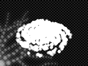 The background image is a sprite that only contains grayscale values. It doesn't use the usual RGBA format for that – the grayscale values are stored directly in the 32-bit words, so the sprite »looks« it's drawn in red. The galaxy is made of 3D transformed point sprites that are drawn using the »add« mode, producing values that are way above the original 8 bits. A final post-processing steps converts the »flat« grayscale values into RGBA grayscale as expected by the display routine. Clipping the overbright values into the (0..255) range is also done in this process.
Scene 2: Planet
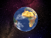 This scene uses a simple raycasting engine: for each screen pixel, the point of collision with the sphere is computed and then transformed from (x, y, z) into polar (latitude, longitude) form. These values are then used to pick the proper texture pixel. The texture is an old, but nice NASA image of the whole earth surface, mapped suitably for polar coordinates. I added some clouds to it to generate a more realistic look.
The main problem with this scene was the transformation into polar coordinates: Among others, it requires an atan2() operation, which is a quite complicated function in my implementation. This function is build of three nested if/then/else statements to decide in which of the 8 half-quadrants (45-degree segments) the arguments are. The result is then computed with a short (0..1)->(0..pi/4) arctan table. Combined with an additional arcuscosine computation (again a table access, expensive on the nano!), this severly degrades performance. When doing the timing, I was glad that the planet scene has such a small timeframe that I could cut it just before it really starts to become jerky.
Scene 3: Mountains
 The only scene in the whole demo that is made entirely with polygon 3D. It is a simplified remake of a scene from my favorite TBL demo, Silkcut. The landscape was made with Terragen. The height map is hand-drawn using Terragen's built-in editor. Afterwards, I exported it as a small 11x11 bitmap. In the demo, the landscape is made up of 10x10 quads whose vertex Z coordinates are taken from the bitmap. The texture is again taken from Terragen. Since the program doesn't actually support exporting the texture, I simply put a camera with a huge focal length several hundred miles above the center of the landscape patch. Then I rendered the image, cropped it appropriately and stored the result in a 256x256 sprite.
I had a really hard time with this scene. It took hours to chose a camera path and fine-tune some additional hacks so that no larger artifacts (from the bad, clipping-less 3D engine) are visible. Since the polygon filler is a little bit »lazy« in that it doesn't draw all of the edge pixels, the contours of the polygons are not completely visible. I hid this effect by simply not clearing the framebuffer between frames. This way, the missing pixels at least contained colors that somewhat resembled the correct ones. In addition, a large sprite was put in the upper-right corner of the screen, because the scene wasn't large enough, and tearing-like artifacts would have been visible in that corner. To sum this up, the whole scene is nothing but a dirty hack.
Scene 4: Wobble
 There's not much to say about this scene: It's just a dual-sine wobble effect with an unanimated image. Due to optimization, the wobbler only draws 128 of the 132 screen lines (this way, wrapping the image is much easier), so an additional hard-alpha sprite is put at the bottom of the screen.
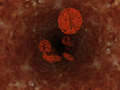
Scene 5: Blood
 This scene is a composite of two completely different, but synchronized effects: A tunnel effect that draws the walls of the blood vessel, and polygon 3D for the blood cells (slow as hell!). The cells are simply low-polygon torii with a primitive texture. The tunnel is again a raycasting effect: This time, the coordinates (x, y, z) of the intersection between the eye ray and the walls (i.e. the cylinder) are transformed into a (phi, z) pair that act as texture coordinates. From the raycasting point of view, the scene isn't animated: The rays will always hit the same spots of the surrounding cylinder. For this reason, all the computations (including the atan2() to get the phi value) are done only once during preparation and stored in a 2D table. The frame rendering loop just takes each pixel's (phi, z) coordinates from the table and uses them as texture coordinates. To simulate animation, the coordinates are translated prior to the texture lookup.
To give the whole scene more depth, a nifty post-processing effect is applied after both the walls and the cells have been drawn: Each pixel's color values are multiplied by its Z value. This makes remote pixels appear darker than close ones, which makes up for a sufficiently convincing 3D effect.
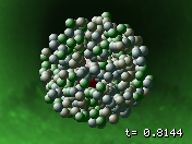
Scene 6: Cells
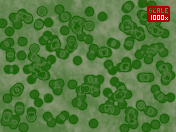 This was the first effect that has been finished, and it's also one of the simplest. Like the galaxy scene, everything is rendered in a pure 32-bit format without separate RGBA bitfields. The cells are actually circular sprites that are added to the static background. A final color mapping process then converts the simple intensity values into the greenish RGBA ones that can be seen on the screen. Overbright values aren't simply clipped, but inverted. This yields funny, somehow organic-looking effects when two or more cells overlap.
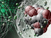
Scene 7: Molecules / Greetings
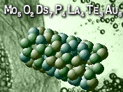 The basic idea of having greetings in the form of (fictional) chemical formulae was one of the first during the design process. I actually wrote a Python script to generate as-real-as-possible formulae from arbitraty words (i.e. those that don't use non-existing element names unless absolutely necessary).
The molecules are rendered as 3D point sprites, with geometry data loaded from disk. The simpler molecules are hand-written (coordinates typed in manually), others are generated. The CNT molecule (carbon nano tube, »cylinder«) is a good example for this. The large fictional molecule at the right end of the scene is generated by starting with one atom and appending new atoms in any of the 6 spatial directions at random. The buckyball (C60 molecule, »sphere«) was tricky, though: I couldn't come up with an easy algorithm to compute the atom coordinates. So I googled a bit and found some Java applets that show these molecules in 3D. After some reverse-engineering, I got hold of the input files for one of these applets and extracted the required coordinates from it.
Scene 8: Electron Microscope
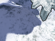
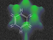 This scene was one of Gabi's first ideas. It is rendered using a simplified voxel engine without perspective mapping. A simple heightmap specifies the displacement (in Y direction) of each pixel. These displacement values are scaled to generate the illusion of varying heights. A fixed color table maps the displacements to display colors. Furthermore, some noise is added it keep the outer areas interesting – they would be a single gray area otherwise.
The Benzene formula that is shown at the top is only made up of half-transparent white lines. The vertex coordinates are computed using a simple 3x2 matrix transform that allows for translation, rotation and scaling in 2D space.
Scene 9: Wilson cloud chamber / Credits
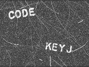 Another effect that uses a pure non-RGBA grayscale representation of the framebuffer internally. However, there's a special twist to it this time: The framebuffer values are re-used after every frame to implement the slowly fading clouds. So the first thing the renderer does is chopping off the green and blue components from the framebuffer values and attenuating the red ones a bit, resulting in nice plain 32-bit intensity values. Furthermore, some slight noise is added to every pixel during this process. Since the amount of fade is dependent on the frame rate, the scene must run with 20-30 fps for optimal visual quality. This is the case on the iPod, but in the PC version, the engine needs to be artificially slowed down for this purpose.
After this pre-conditioning step, the elements of the scene are added one after another (literally added: the pixel values in the frame buffer are incremented).
First, 1000 random pixels will get a random (1/4 max.) intensity gain.
Second, one »gamma ray« with the same maximum intensity will be added per frame. A gamma ray, in the scene's context, is simply a line somewhere on the screen, in any orientation, that crosses the complete screen.
Third, the heavier nucleons traces (20 of them) are drawn. These are slower and react to the chamber's magnetic field, hence they travel along circular paths. From the implementation's point of view, each nucleon has a position and a movement vector. The routine will draw a small line strip with full intensity from the nucleons current position to the position it will have in the next frame (computed by adding the current position and the movement vector). Finally the movement vector will be rotated a bit, which generates the illusion of a circular trajectory. Due to the slow fade of the cloud chamber, these are visible quite well. After a number of frames, a nucleon »dies« and appears elsewhere on the screen.
Finally, the credits are added using sprites with a quickly jittering position.
After all these drawing steps, the screen is again converted from the flat intensity format to the common RGBA one.
Scene 10: Atoms
 This is a very straightforward scene: A background, some point-sprite nucleons and electrons, and some orbital lines. The nucleons' geometry data is loaded from files that have been generated by a (painfully slow :) Python script, based on the number of protons and neutrons in each of the six elements (hydrogen, helium, carbon, silicon, gold and uranium). The electron orbitals are drawn using partially-transparent white lines. They aren't exactly circular, but regular 32-sided polygons, except for the gold and uranium ones: To save processing power, the polygons are only 16-sided for these atoms. Nevertheless, this is the scene that drives the iPod (or rather, my bad programming :) closest to its limits, with down to ~3 fps while the uranium atom is fully shown.
Scene 11: Particle Accelerator / Collision
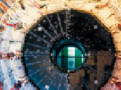 These are in fact two scenes: The first one is a Ken Burns type zoom into the accelerator and the second one is the collision itself, none of which is anything special, technology-wise.
For the introductory scene, I chose an image of the DELPHI detector of the (now dismantled) LEP accelerator at CERN. The effect itself isn't actually worth speaking about: It's basically a rotozoomer, just without the rotation component :)
 The collision scene is again made with 3D-transformed point sprites, so there's not much to say about it, too. The background image is a funny thing, though: It's not even remotely related to particle accelerators – it's a shot inside a mere plastic pipe ...
Scene 12: Kakiarts Logo
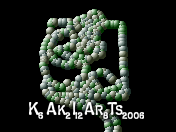 Right from the start, I wanted to have the Kakiarts logo in form of a hyper-complex molecule. To accomplish this, I used a Python script (again) that takes a black/white image and places atoms only in places that map to black pixels. I fed a simplified image of our mascot into the script and voilà, I had a nice 256-atom logo molecule. Unfortunately, the nano screen proved a little bit to small for it – the monkey mascot was hardly recognizable :(
Just before I decided to ditch the molecule monkey altogether, Gabi came up with a brilliant idea: Blend the molecule logo slowly into the normal, bitmapped one. For some extra effect, I let the atoms from the molecule disappear one after another while the bitmap slowly faded from black. I was delighted to see that this just looked gorgeous :) Seemingly, other sceners share this opinion, because that scene is the most frequently praised one ....
I conclude with a little bit of trivia: The last three numbers in the Kakiarts formula at the end (12-8-2006) together form the release date of the demo: August 12, 2006.
How can I install it on my 2Gb Nano using Floyzilla? Reply would be really really kind as I´m very very interested in that demo.
Thanks ;-)
Ha ha! That is truely awesome KeyJ. Thanks for the descriptions – although a little over my head (in parts) it was interesting to read about the work arounds for the ARM7TDMI. And it looks like I’m not the only one using Terragen to generate textures “from above”!! I wish I had have introduced myself at Evoke (I was sitting next to dq) but you guys looked pretty busy. Maybe in 2008 :-)